TensorFlow 2.0 の練習を兼ねて、非負値行列因子分解 (NMF) を実装しました。
問題設定
NMF は非負値行列 $X \in \mathbb{R}^{T \times F}$ を二つの低ランク行列の積 $WH$ で近似するアルゴリズムで、混合音の音源分離などに使われます。ここでは $X$ に混合音のスペクトログラムの絶対値を代入し、$K$ 種類の音 $H \in \mathbb{R}^{K \times F}$ とその出現パターン $W \in \mathbb{R}^{T \times K}$ を分析します。
$T$ は時間フレーム数、$F$ は周波数ビンの数をあらわします。
Adam による勾配法を実装するため、$X$ と $WH$ の乖離度を定義します。ここでは、二乗誤差と I-ダイバージェンスを実装しました。
$W$ と $H$ の推定値がマイナスになると厄介なので、今回は $\ln W$ と $\ln H$ を推定します。
ソースコード
import librosa
import numpy as np
import tensorflow as tf
from matplotlib import pyplot as pl
from matplotlib.gridspec import GridSpec

# librosa を使い、wav ファイルを読み込みます。
# 今回はサンプルなので、読み込み時のオプションはあまり設定しないことにします。
# 信号のサンプリングレートはデフォルトで 22.5kHz に変換されます。
#
# 楽曲全体を NMF にかけるとかなりの時間がかかるので、先頭 30 秒だけを分析します。
# 信号は絶対値の平均値が 1 となるよう正規化しておきます。
nsecond = 30
sig, fs = librosa.load('sample.wav', mono=True)
sig = sig[:fs * nsecond]
sig_stft = abs(librosa.stft(sig).T)
sig_stft /= sig_stft.mean()

# T: nframe, F: nbin, K: 20 に設定します。
nbasis = 20
nframe, nbin = sig_stft.shape

# TensorFlow の定数と変数を定義します。対数を計算する際のゼロ除算を避けるため、
# あらかじめ微小量 (1e-10) を加えておきます。
#
# lw (ln W), lh (ln H) は Adam で更新するため、tf.Variable で宣言します。
# 初期値には特にこだわりがないのですが、ここでは正規分布で初期化します。
x = tf.constant(sig_stft + 1e-10)
lx = tf.constant(tf.math.log(x))
lw = tf.Variable(tf.random.normal([nframe, nbasis]))
lh = tf.Variable(tf.random.normal([nbasis, nbin]))

# グラフを準備します。乖離度 (loss), W, H, WH のための subplot を作ります。
fig = pl.figure(constrained_layout=True)
gs = GridSpec(5, 5, figure=fig)
axl = fig.add_subplot(gs[0, 0])
axw = fig.add_subplot(gs[0, 1:])
axh = fig.add_subplot(gs[1:, 0])
axs = fig.add_subplot(gs[1:, 1:])

# オプティマイザを作成します。Adam のデフォルトの学習率は 0.001 ですが、
# NMF は 0.1 でも動作しました。逆に、これ位にしないと学習時間がかかりすぎるようです。
# ニューラルネットに比べて loss の複雑度が低いのかもしれません。
opt = tf.keras.optimizers.Adam(learning_rate=.1)

history = []
for i in range(10000):
    # loss を定義します。この関数は引数なしとする必要があります。
    def loss_euc():
        wh = tf.matmul(tf.exp(lw), tf.exp(lh))
        return tf.reduce_sum((x - wh) ** 2)
    def loss_idiv():
        lwh = tf.reduce_logsumexp(lw[:, :, None] + lh[None, :, :], axis=1)
        return tf.reduce_sum(x * (lx - lwh - 1) + tf.exp(lwh))

    # Adam で変数の値を更新します。
    # var_list に更新したい変数 (tf.Variable) を指定します。
    opt.minimize(loss_idiv, var_list=[lw, lh])

    # 現在の loss の値を計算します。
    history.append(np.log(loss_idiv().numpy()))

    # イテレーション毎にグラフを表示します。
    axl.clear()
    axw.clear()
    axh.clear()
    axs.clear()
    axl.set_xticks([0, i])
    axl.set_yticks([np.array(history).min(), np.array(history).max()])
    axw.set_xticks([0, nframe - 1])
    axw.set_yticks([0, nbasis - 1])
    axh.set_xticks([0, nbasis - 1])
    axh.set_yticks([0, nbin - 1])
    axs.set_xticks([0, nframe - 1])
    axs.set_yticks([0, nbin - 1])

    # グラフのカラースケールを固定するため、1e-3 (-60dB) で足切りします。
    wh = tf.matmul(tf.exp(lw), tf.exp(lh)).numpy()
    lw_display = tf.maximum(lw, tf.reduce_max(lw) + np.log(1e-3)).numpy()
    lh_display = tf.maximum(lh, tf.reduce_max(lh) + np.log(1e-3)).numpy()
    lwh_display = np.log(np.maximum(wh, wh.max() * 1e-3))

    axl.plot(history)
    axw.imshow(lw_display.T, aspect='auto')
    axh.imshow(lh_display.T, aspect='auto', origin='lower')
    axs.imshow(lwh_display.T, aspect='auto', origin='lower')
    pl.pause(.1)
実行結果
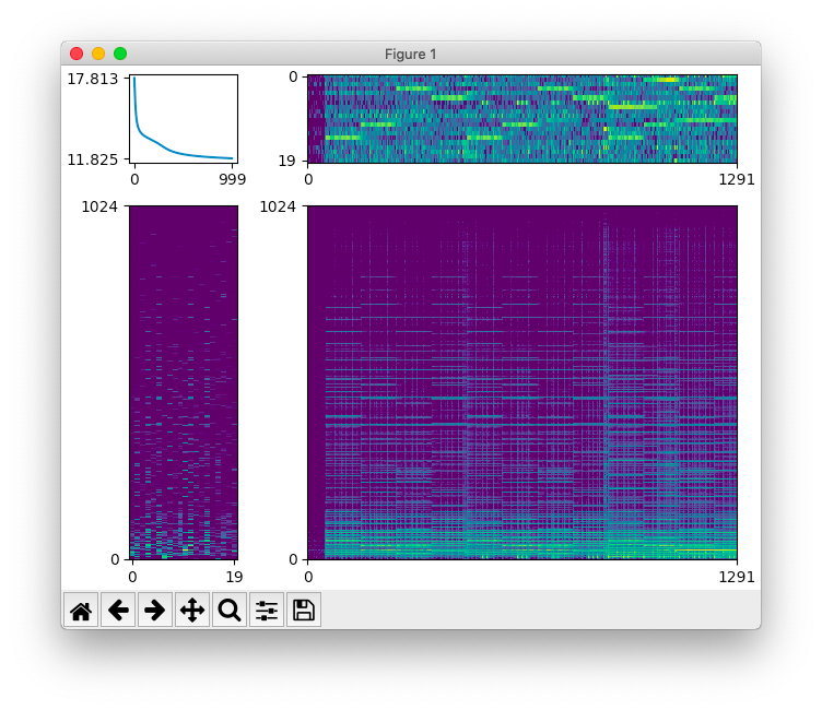
上のスクリプトの実行結果です。 $W$ (右上)と $H$ (左下)が推定できています。 右下に表示しているのは NMF による再構築結果 $WH$ です。
動作環境は macOS Mojave (10.14) + TensorFlow 2.0.0b1 です。
参考文献
-
TensorFlow
https://www.tensorflow.org/ -
tf.keras.optimizers.Optimizer | TensorFlow Core r2.0
https://www.tensorflow.org/versions/r2.0/api_docs/python/tf/keras/optimizers/Optimizer -
tf.keras.optimizers.Adam | TensorFlow Core r2.0
https://www.tensorflow.org/versions/r2.0/api_docs/python/tf/keras/optimizers/Adam -
Librosa
https://librosa.github.io/ -
非負値行列因子分解
http://www.kecl.ntt.co.jp/people/kameoka.hirokazu/publications/Kameoka2012SICE09published.pdf